Data Visualization
With the BiofilmQ visualization tab you can create publication-quality figures of your measurements.
Quick Start
Load data into the visualization process by navigating to the experiment folder you would like to analyze, and then click the Load data-button.
Select in the Options-panel the desired plot type.
Add parameters to the axes by first selecting them in the Parameter selection-panel and then using the small + next to the desired axis.
When no axis is colored red, you can start plotting by using the Plot button in the bottom right corner.
Note
By default figures are automatically stored inside /data/evaluation in the FIG, EPS and PNG format files with readable labels.
Step-by-Step
Import data
When you first open the visualization tab, it is completely empty. To directly interact with the data (and to quickly generate plots) you have to load data into the workspace. You can load data into the visualization process by navigating to the experiment folder you would like to analyze, and then click the Load data-button.
Options:
Subtract reference time point can be used to change the time reference point. Example: Show a reporter activity over time only after a certain biofilm size is reached. * Step 1: Plot biofilm size over time. * Step 2: Select in the drop down menu next to Subtract reference time point the time (i.e. image frame) when the desired size is reached. All following time points will be shifted according to this reference frame.
Fluorescence channel to load define the channel which you want to analyze (assuming segmented data files are present for that channel).
Limit maximum frame number If your time series are quite large, but you are only interested in the biofilm development until a certain point, you can limit the amount of data which is loaded into memory by enabling this checkbox.
Parameter selection
The parameter selection panel can be used to conveniently select interesting biofilm parameters that can be assigned to an axis of the figure.
Note that you can change the parameter list from Single object parameters to Global biofilm parameters in the drop-down menu at top left of the panel.
At the top right you can search the parameters by name. By pressing Enter on your keyboard, you can invoke the search.
Similar global biofilm parameters are grouped. You can expand a grouped set by clicking on [+] in front of the group. A group includes the following global measures per single-object parameter:
max
mean
mean_biovolume (weighted by object volume)
median
min
p25 (25th percentile)
p75 (75th percentile)
std (standard deviation)
std_biovolume (standard deviation, weighted by object volume)
once the parameter distanceToCenterOfBiofilm was calculated, parameters with additional suffixes are available:
core (i.e. parameters with the core-suffix in the name). All objects closer than half of the 90% percentile distance of all objects to the center of the biofilm.
shell (i.e. parameters with the shell-suffix in the name). All objects further away than half of the 90% percentile distance of all objects to the center of the biofilm.
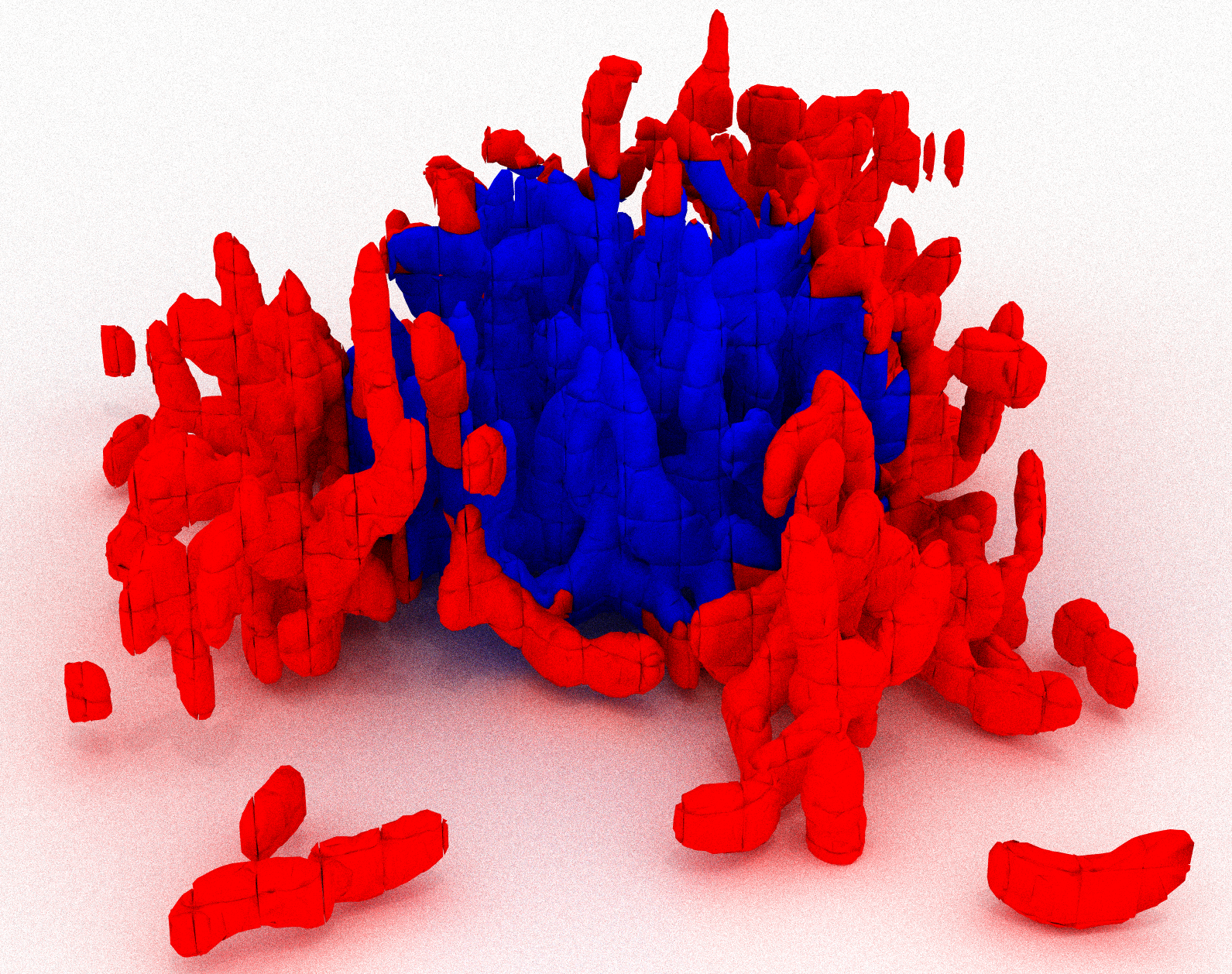
Example of shell and core cubes. Core cubes are colored in blue, shell cubes are colored in red.
Plotting options
The Options panel is designed in such a way that depending on the plot type different input options can be selected.
Regardless of the selected plot type, you can assign parameters to different axes (depending on the plot type: \(x\), \(y\), \(z\), and color). Each axis has several input fields:
Parameter Internal name of the calculated biofilm parameter.
Label Axis label in the plot figure.
Unit Defines which unit name is used in the figure label.
AR (Auto-Range) Enables/ disables the manual range settings for the plot axis.
Range either manually defined range, or the hard-coded range based on the parameter type.
TR (True-Range) Enables/ disables a range lookup of the calculated parameter to adapt to the actual data range.
Method Sets the method (min/max, 1-99th percentile) for the True-Range-lookup.
Bins (3D Heatmap, Histogram only) defines how many bins should be used for the axis.
Log Enables/ disables logarithmic scaling for this axis.
Note
You can quickly transfer the selected parameter from the Parameter selection with the small +-button next to the parameter-textbox.
If you can not see any markers in you plot. Check whether your Range settings are correct.
Additional options
If you enable the Interpolate data points for missing cell numbers-checkbox the global parameter cell_number is interpolated between the measured time points. This option can be useful if you want to use the cell_number instead of time to measure the developmental state of the biofilm.
Method (only 3D Heatmap, 2D XY-Plot per frame, and 1.5D Histogram) defines how the plotted parameter value is calculated.
Mean (weighted by object volume) \(\pm\) weighted standard deviation
Mean \(\pm\) standard deviation
Median \(\pm\) upper/ lower quartile
Sum
Min
Max
Note
- If the biofilm was dissected using the cube method, averaging of cube-based parameters is biased by the actual volume
present in each cube. To put less weight on hardly-filled cubes, you can either calculate mean values that are weighted by volume in each cube, or you can remove cubes with a very small volume fraction (i.e. less than 0.05).
Style (only 2D XY-Plot per frame, Histogram) modifies the marker style of the given plots.
Plot error bars (only 2D XY-Plot per frame and 1.5D Histogram) enables/ disables error bars in the plot.
Heatmap options
On the right-hand side you can find the Heatmap options, which modifies the selected plot (3D Heatmap only).
Y offset Shifts the calculated parameter the given amount in \(y\) direction.
Normalize by Divides the heatmap tiles by the given number.
Remove global z-offset (only if d_z is parameter in 3D Heatmap or z in all other plot types except 2D histogram) subtracts the minimal value in d_z/z from the d_z/z before plotting.
Remove z-offset per heatmap column Removes in each column NaN values until the first data value is reached. Modifies value such that column starts with valid data point
Invert Y-axis Switches from a ascending to a descending \(y\) axis.
Note
Y-offset correction options are meant to correct heatmaps of time series with slight shifts in focus positions only!
Actions
Use Plot-button to create a plot based on the previously selected options. Additionally you can:
Save plots as png and eps files Save the figures as MATLAB FIG-file, as bitmap PNG file and in the eps vector graphics format. The figures will be saved in the subfolder data/evaluation of the current Experiment folder. The name of the plots will be based on the plot type and the plotted parameters.
Overwrite existing files If the first option is checked, the already saved plots are not overwritten unless this option is enabled.
Add plot to current figure If you want to accumulate data in a single plot you can use this option.
Note
Creating eps figures with a large number of elements (i.e. scatter plots) can take a long time.
If you accumulate data in a single plot, the axis labels and the plot range will be set according to the most recently added data. If you want to use multiple axis label, you have to modify the plot manually.
Plot types
Tutorials provide examples of and details on the different plot types.
Histogram plots (1D and 1.5D)
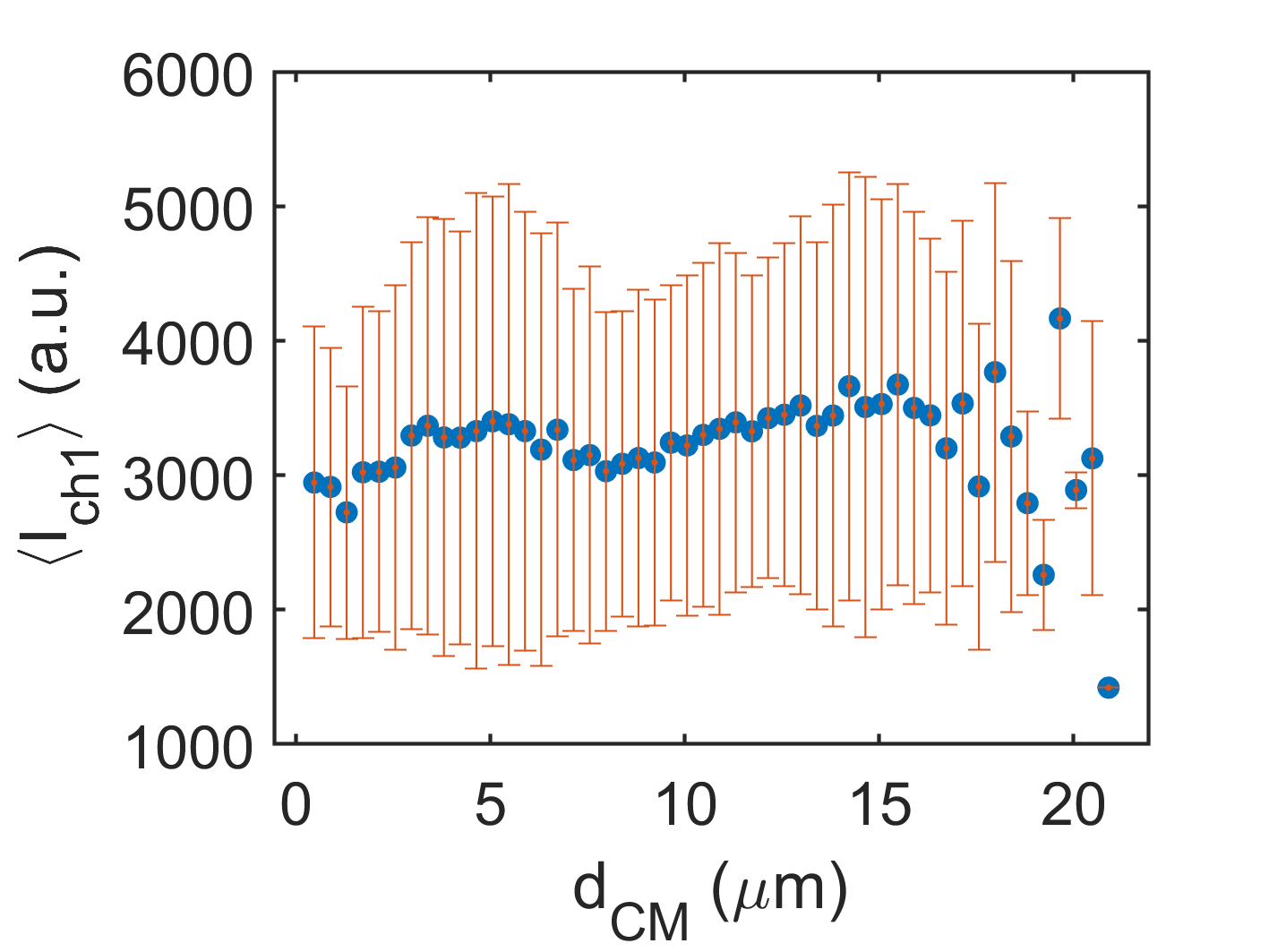
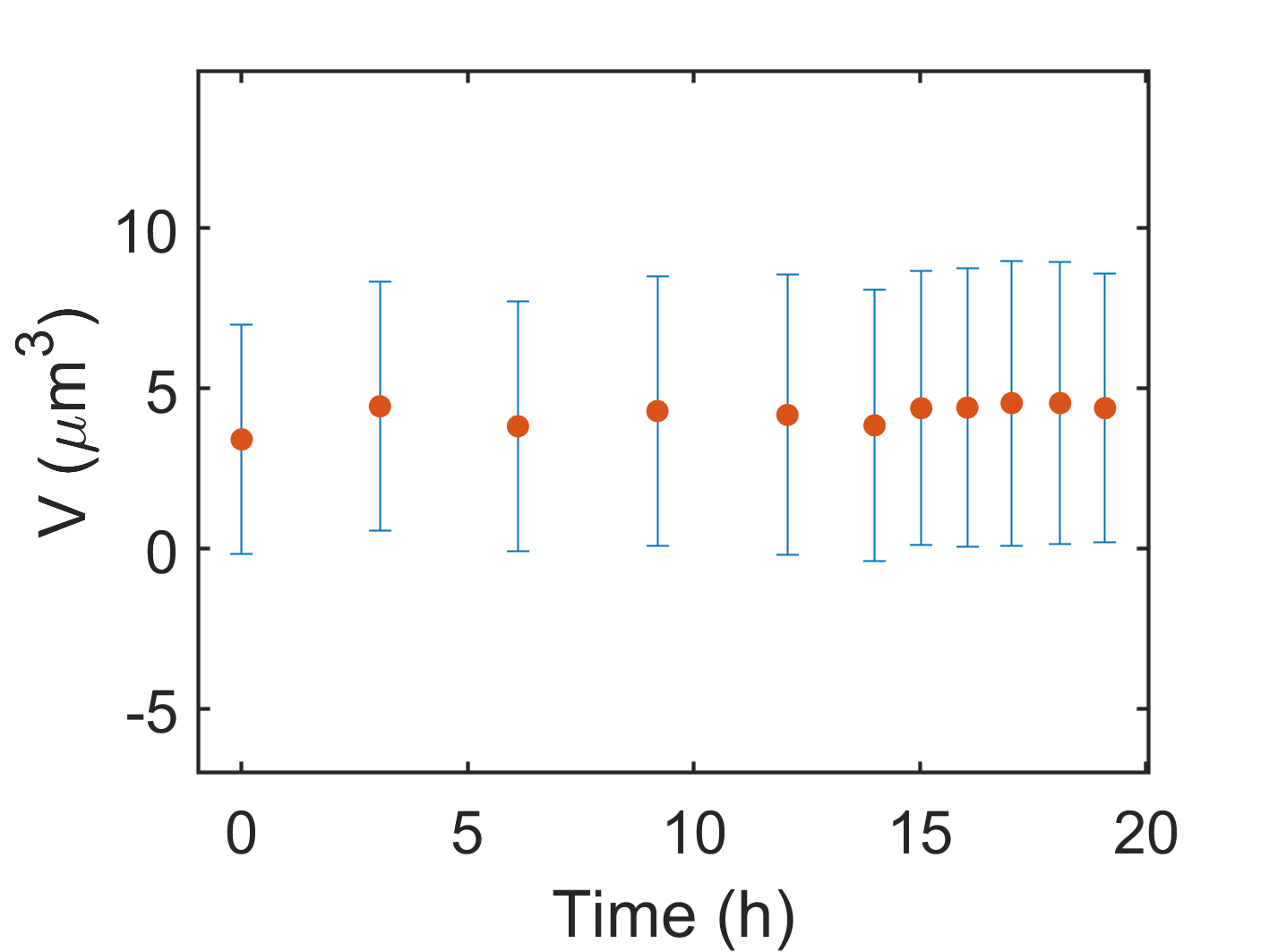
2D XY Plot per frame
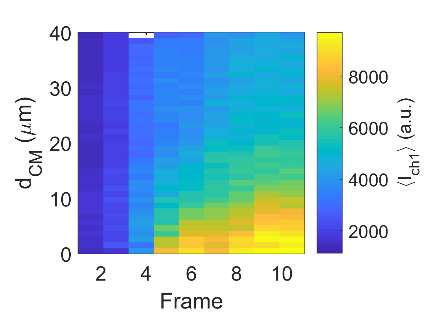
Kymograph and Demograph plots
Scatter plots (2D and 4D)
Filtering/ Gating
Analogous to flow cytometry, BiofilmQ offers the ability to apply gates/ filters to your data, to analyze separate subpopulations of your data separately. If you want to use only a subset of the calculated data, you can use the filtering field to define multiple conditions before plotting the data. Filtering does not work with global parameters.
A valid filtering conditions consists of a calculated parameter (i.e. Volume), an operator (i.e.: >, <, <=, >=, ==, ~=, see `MATLAB comparison operators <https://de.mathworks.com/help/matlab/matlab_prog/array-comparison-with-relational-operators.html>`_), and a numeric value. Multiple conditions can be joined with logical operator (i.e.: *| (or), & (and), see `MATLAB logical operatorsy <https://de.mathworks.com/help/matlab/matlab_prog/matlab-operators-and-special-characters.html>`_ ). Next to the Filtering / Gating text field you find a small + button which can be used to add the currently selected parameter to the filtering rule.
Note
- If the biofilm was dissected using the cube method, averaging of cube-based parameters is biased by the actual
biomass present in each cube. To put less weight on hardly-filled cubes, you can either calculate mean values that are weighted by the volume of each cube, or you can remove cubes with a very small volume fraction (i.e. less than 0.05)
Advanced options
In case the BiofilmQ build-in functionality for data visualization might not be sufficient for all visualization ideas you have in mind, you can use custom scripts before plotting (i.e. custom data analysis) (Apply custom script on data) or modification of the already plotted figure with the checkbox Apply custom script on plot (i.e. to change the plot colors etc.)
You can find example scripts in the BiofilmQ source folder under includes/biofilm analysis/custom scripts.
Color 2D scatter plots by point density
Coloring 2D scatter points by point density is implemented as a custom script (as it has many input parameters). Check Apply custom script on plot and browse for the corresponding script in the default custom script folder.
Example Plots
3D Heatmap/Kymograph
2D XY-Plot per frame
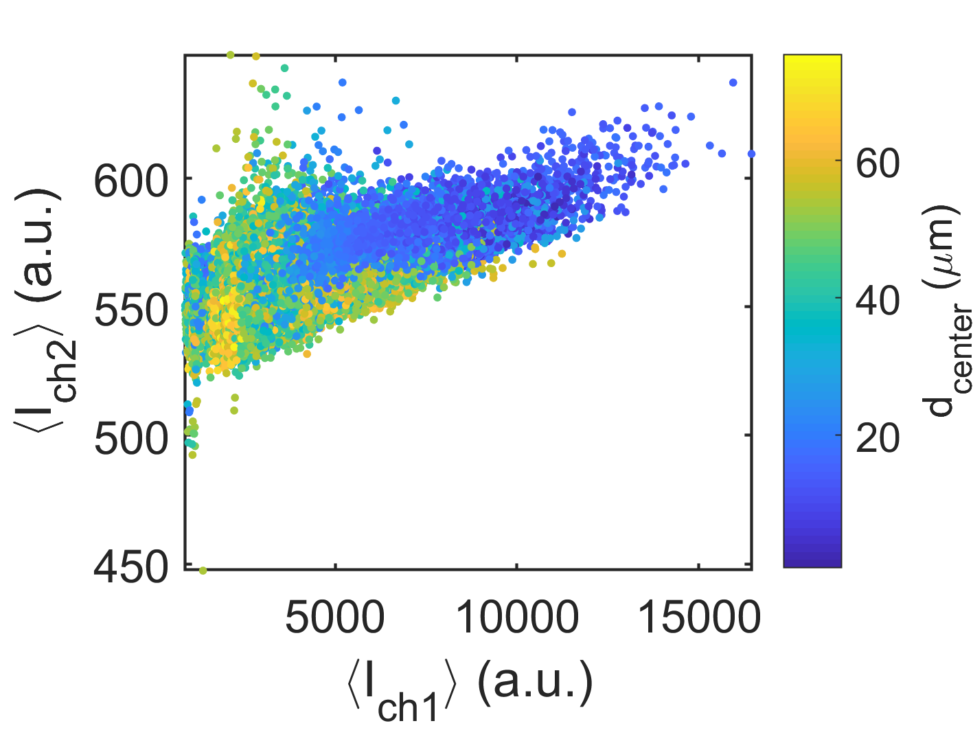
2D XY-Scatterplot
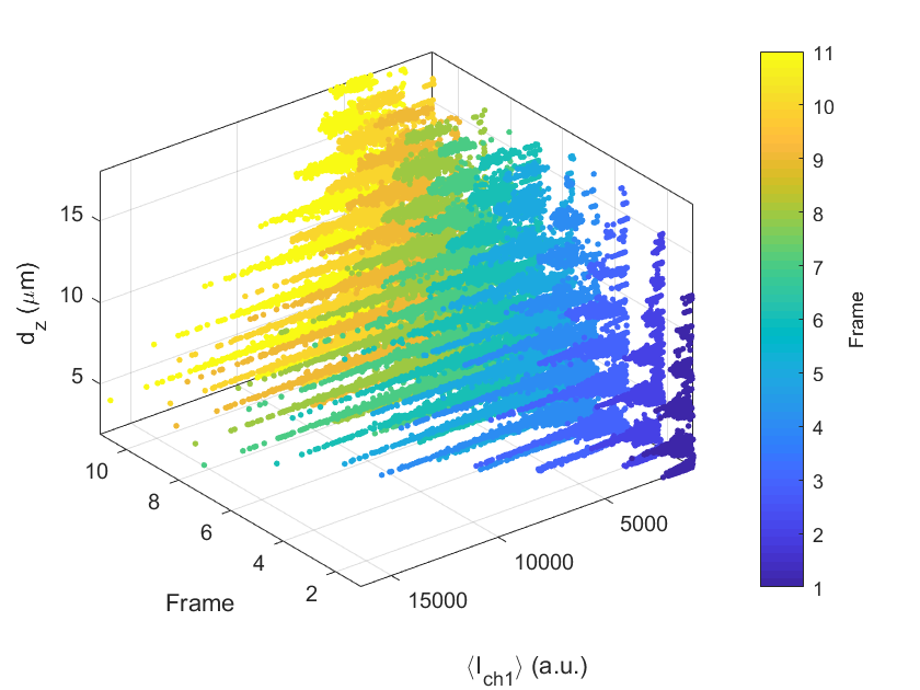
4D XYZC-Scatterplot
1D Histogram

1.5D Histogram